Math and array tools

Arrays are the basis of science [citation needed]. This tutorial walks you through some tools to make your life working with arrays a little more pleasant.

Click here to open an interactive version of this notebook.

Array indexing

Let’s create some data.

import numpy as np

data = np.random.rand(100)

print(f'{data = }')

data = array([0.96702984, 0.54723225, 0.97268436, 0.71481599, 0.69772882,
       0.2160895 , 0.97627445, 0.00623026, 0.25298236, 0.43479153,
       0.77938292, 0.19768507, 0.86299324, 0.98340068, 0.16384224,
       0.59733394, 0.0089861 , 0.38657128, 0.04416006, 0.95665297,
       0.43614665, 0.94897731, 0.78630599, 0.8662893 , 0.17316542,
       0.07494859, 0.60074272, 0.16797218, 0.73338017, 0.40844386,
       0.52790882, 0.93757158, 0.52169612, 0.10819338, 0.15822341,
       0.54520265, 0.52440408, 0.63761024, 0.40149544, 0.64980511,
       0.3969    , 0.62391611, 0.76740497, 0.17897391, 0.37557577,
       0.50253306, 0.68666708, 0.25367965, 0.55474086, 0.62493084,
       0.89550117, 0.36285359, 0.63755707, 0.1914464 , 0.49779411,
       0.1824454 , 0.91838304, 0.43182207, 0.8301881 , 0.4167763 ,
       0.90466759, 0.40482522, 0.3311745 , 0.57213877, 0.84544365,
       0.86101431, 0.59568812, 0.08466161, 0.59726661, 0.24545371,
       0.73259345, 0.89465129, 0.51473397, 0.60356351, 0.06506781,
       0.54007473, 0.12918678, 0.61456285, 0.36365035, 0.76775803,
       0.04853414, 0.10981812, 0.68402322, 0.5146537 , 0.57164137,
       0.84370699, 0.48773764, 0.81014442, 0.51024363, 0.92672069,
       0.66692777, 0.14872684, 0.36455318, 0.86577492, 0.35028521,
       0.18902576, 0.47262131, 0.39278117, 0.61892993, 0.43676629])

What if we want to do something super simple, like find the indices of the values above 0.9? In NumPy, it’s not super straightforward:

inds = (data>0.9).nonzero()[0]

print(f'{inds = }')

inds = array([ 0,  2,  6, 13, 19, 21, 31, 56, 60, 89])

In Sciris, there’s a function for doing exactly this:

import sciris as sc

inds = sc.findinds(data>0.9)

print(f'{inds = }')

inds = array([ 0,  2,  6, 13, 19, 21, 31, 56, 60, 89])

Likewise, what if we want to find the value closest to, say, 0.5? In NumPy, that would be

target = 0.5
nearest = np.argmin(abs(data-target))

print(f'{nearest = }, {data[nearest] = }')

nearest = 54, data[nearest] = 0.4977941146173057

Which is not too long, but it’s a little harder to remember than the Sciris equivalent:

nearest = sc.findnearest(data, target)

print(f'{nearest = }, {data[nearest] = }')

nearest = 54, data[nearest] = 0.4977941146173057

The Sciris functions also work on anything “data like”: for example,

target = 50
data = [81, 78, 66, 25,  6,  8, 53, 96, 64, 23]

# With NumPy
ind = np.argmin(abs(np.array(data)-target))

# With Sciris
ind = sc.findnearest(data, 50)

print(f'{ind=}, {data[ind]=}')

ind=6, data[ind]=53

These have been simple examples, but you can see how Sciris functions can do the same things with less typing.

Interlude on creating arrays

Speaking of which, here’s a pretty fast way to create an array:

sc.cat(1,2,3)

array([1, 2, 3])

sc.cat() will take anything array-like and turn it into an actual array. For example:

# Create a 2x2 matrix
data = np.random.rand(2,2)

# Add a row with NumPy
data = np.concatenate([data, np.atleast_2d(np.array([1,2]))])

# Add a row with Sciris
data = sc.cat(data, [1,2])

print(f'{data = }')

data = array([[0.26092216, 0.41247221],
       [0.41903403, 0.90242186],
       [1.        , 2.        ],
       [1.        , 2.        ]])

Yes, the NumPy command really does end with ]))]).

Missing values

Now that we know some tools for indexing arrays, let’s look at ways to actually change them.

We all know that missing data is one of humanity’s greatest scourges. Luckily, it can be swiftly eradicated with Sciris: either removed entirely or replaced:

d0 = [1, 2, np.nan, 4, np.nan, 6, np.nan, np.nan, np.nan, 10]

d1 = sc.rmnans(d0) # Remove nans
d2 = sc.fillnans(d0, 0) # Replace NaNs with 0s
d3 = sc.fillnans(d0, 'linear') # Replace NaNs with linearly interpolated values

print(f'{d0 = }')
print(f'{d1 = }')
print(f'{d2 = }')
print(f'{d3 = }') # This is more impressive than ChatGPT, imo

d0 = [1, 2, nan, 4, nan, 6, nan, nan, nan, 10]
d1 = array([ 1.,  2.,  4.,  6., 10.])
d2 = array([ 1.,  2.,  0.,  4.,  0.,  6.,  0.,  0.,  0., 10.])
d3 = array([ 1.,  2.,  3.,  4.,  5.,  6.,  7.,  8.,  9., 10.])

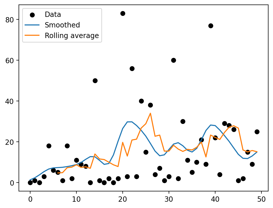
Data smoothing

What if we have some seriously lumpy data we want to smooth out? We have a few options for doing that:

# Make data
n = 50
x = np.arange(n)
data = 20*np.random.randn(n)**2
data = sc.randround(data) # Stochastically round to the nearest integer -- e.g. 0.7 is rounded up 70% of the time

# Simple smoothing
smooth = sc.smooth(data, 7)

# Use a rolling average
roll = sc.rolling(data, 7)

# Plot results
import pylab as pl
sc.options(jupyter=True)
pl.scatter(x, data, c='k', label='Data')
pl.plot(x, smooth, label='Smoothed')
pl.plot(x, roll, label='Rolling average')
pl.legend();

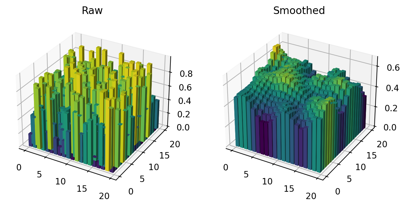
We can also smooth 2D data:

# Create the data
raw = pl.rand(20,20)

# Smooth it
smooth = sc.gauss2d(raw, scale=2)

# Plot
fig = pl.figure(figsize=(8,4))

ax1 = sc.ax3d(121)
sc.bar3d(raw, ax=ax1)
pl.title('Raw')

ax2 = sc.ax3d(122)
sc.bar3d(smooth, ax=ax2)
pl.title('Smoothed');

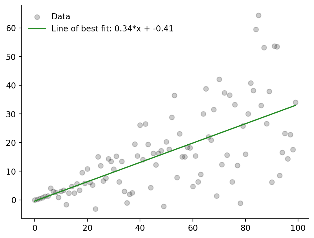
Finding a line of best fit

It’s also easy to do a very simple linear regression in Sciris:

# Generate the data
n = 100
x = np.arange(n)
y = x*np.random.rand() + 0.2*np.random.randn(n)*x

# Calcualte the line of best fit
m,b = sc.linregress(x, y)

# Plot
pl.style.use('sciris.simple')
pl.scatter(x, y, c='k', alpha=0.2, label='Data')
pl.plot(x, m*x+b, c='forestgreen', label=f'Line of best fit: {m:0.2f}*x + {b:0.2f}')
pl.legend();