Advanced features

Here are yet more tools that the average user won’t need, but might come in handy one day.

Click here to open an interactive version of this notebook.

Nested dictionaries

Nested dictionaries are a useful way of storing complex data (and in fact are more or less the basis of JSON), but can be a pain to interact with if you don’t know the structure in advance. Sciris has several functions for working with nested dictionaries. For example:

import sciris as sc

# Create the structure
nest = {}
sc.makenested(nest, ['key1','key1.1'])
sc.makenested(nest, ['key1','key1.2'])
sc.makenested(nest, ['key1','key1.3'])
sc.makenested(nest, ['key2','key2.1','key2.1.1'])
sc.makenested(nest, ['key2','key2.2','key2.2.1'])

# Set the value for each "twig"
count = 0
for twig in sc.iternested(nest):
    count += 1
    sc.setnested(nest, twig, count)

# Convert to a JSON to view the structure more clearly
sc.printjson(nest)

# Get all the values from the dict
values = []
for twig in sc.iternested(nest):
    values.append(sc.getnested(nest, twig))
print(f'{values = }')

{
  "key1": {
    "key1.1": 1,
    "key1.2": 2,
    "key1.3": 3
  },
  "key2": {
    "key2.1": {
      "key2.1.1": 4
    },
    "key2.2": {
      "key2.2.1": 5
    }
  }
}
values = [1, 2, 3, 4, 5]

Sciris also has a sc.search() function, which can find either keys or values that match a certain pattern:

print(sc.search(nest, 'key2.1.1'))
print(sc.search(nest, value=5))

[['key2', 'key2.1', 'key2.1.1']]
[['key2', 'key2.2', 'key2.2.1']]

There’s even an sc.iterobj() function that can make arbitrary changes to an object:

def increment(obj):
    return obj + 1000 if isinstance(obj, int) and obj !=3 else obj

sc.iterobj(nest, increment, inplace=True)
sc.printjson(nest)

{
  "key1": {
    "key1.1": 1001,
    "key1.2": 1002,
    "key1.3": 3
  },
  "key2": {
    "key2.1": {
      "key2.1.1": 1004
    },
    "key2.2": {
      "key2.2.1": 1005
    }
  }
}

Context blocks

Sciris contains two context block (i.e. “with ... as”) classes for catching what happens inside them.

sc.capture() captures all text output to a variable:

import sciris as sc
import numpy as np

def verbose_func(n=200):
    for i in range(n):
        print(f'Here are 5 random numbers: {np.random.rand(5)}')

with sc.capture() as text:
    verbose_func()

lines = text.splitlines()
target = '777'
for l,line in enumerate(lines):
    if target in line:
        print(f'Found target {target} on line {l}: {line}')

Found target 777 on line 37: Here are 5 random numbers: [0.23091441 0.92720101 0.64386704 0.98108182 0.77739743]
Found target 777 on line 40: Here are 5 random numbers: [0.10017502 0.85447773 0.70585521 0.79761481 0.56303318]
Found target 777 on line 42: Here are 5 random numbers: [0.98338691 0.23776133 0.79377702 0.38521457 0.13102052]
Found target 777 on line 57: Here are 5 random numbers: [0.48547204 0.0794115  0.83758695 0.59309727 0.48170777]
Found target 777 on line 128: Here are 5 random numbers: [0.91227649 0.17771961 0.64710676 0.36414018 0.0829745 ]

The other function, sc.tryexcept(), is a more compact way of writing try ... except blocks, and gives detailed control of error handling:

def fickle_func(n=1):
    for i in range(n):
        rnd = np.random.rand()
        if rnd < 0.005:
            raise ValueError(f'Value {rnd:n} too small')
        elif rnd > 0.99:
            raise RuntimeError(f'Value {rnd:n} too big')

sc.heading('Simple usage, exit gracefully at first exception')
with sc.tryexcept():
    fickle_func(n=1000)

sc.heading('Store all history')
tryexc = None
for i in range(1000):
    with sc.tryexcept(history=tryexc, verbose=False) as tryexc:
        fickle_func()
tryexc.disp()

————————————————————————————————————————————————
Simple usage, exit gracefully at first exception
————————————————————————————————————————————————

<class 'RuntimeError'> Value 0.995604 too big


—————————————————
Store all history
—————————————————

                      type                        value                             traceback
0   <class 'RuntimeError'>       Value 0.992427 too big  <traceback object at 0x7f3430157a80>
1     <class 'ValueError'>    Value 0.0035279 too small  <traceback object at 0x7f3428df4a80>
2   <class 'RuntimeError'>       Value 0.991026 too big  <traceback object at 0x7f3402fa3a80>
3   <class 'RuntimeError'>       Value 0.996673 too big  <traceback object at 0x7f3402eb74c0>
4     <class 'ValueError'>  Value 0.000397334 too small  <traceback object at 0x7f3402eb7400>
5   <class 'RuntimeError'>       Value 0.992735 too big  <traceback object at 0x7f3402eb7140>
6   <class 'RuntimeError'>       Value 0.995062 too big  <traceback object at 0x7f3402eb76c0>
7   <class 'RuntimeError'>       Value 0.992525 too big  <traceback object at 0x7f3402eb7540>
8   <class 'RuntimeError'>       Value 0.993638 too big  <traceback object at 0x7f3402eb6f00>
9     <class 'ValueError'>     Value 0.001585 too small  <traceback object at 0x7f3402eb7800>
10    <class 'ValueError'>   Value 0.00207436 too small  <traceback object at 0x7f3402eb7300>
11  <class 'RuntimeError'>       Value 0.996381 too big  <traceback object at 0x7f3402eb7880>

Interpolation and optimization

Sciris includes two algorithms that complement their SciPy relatives: interpolation and optimization.

Interpolation

The function sc.smoothinterp() smoothly interpolates between points but does not use spline interpolation; this makes it somewhat of a balance between numpy.interp() (which only interpolates linearly) and scipy.interpolate.interp1d(..., method='cubic'), which takes considerable liberties between data points:

import sciris as sc
import numpy as np
import pylab as pl
from scipy import interpolate

# Create the data
origy = np.array([0, 0.2, 0.1, 0.9, 0.7, 0.8, 0.95, 1])
origx = np.linspace(0, 1, len(origy))
newx  = np.linspace(0, 1)

# Create the interpolations
sc_y = sc.smoothinterp(newx, origx, origy, smoothness=5)
np_y = np.interp(newx, origx, origy)
si_y = interpolate.interp1d(origx, origy, 'cubic')(newx)

# Plot
kw = dict(lw=2, alpha=0.7)
pl.plot(newx, np_y, '--', label='NumPy', **kw)
pl.plot(newx, si_y, ':',  label='SciPy', **kw)
pl.plot(newx, sc_y, '-',  label='Sciris', **kw)
pl.scatter(origx, origy, s=50, c='k', label='Data')
pl.legend();

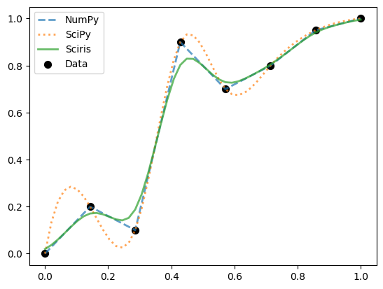
As you can see, sc.smoothinterp() gives a more “reasonable” approximation to the data, at the expense of not exactly passing through all the data points.

Optimization

Sciris includes a gradient descent optimization method, adaptive stochastic descent (ASD), that can outperform SciPy’s built-in optimization methods (such as simplex) for certain types of optimization problem. For example:

# Basic usage
import numpy as np
import sciris as sc
from scipy import optimize

# Very simple optimization problem -- set all numbers to 0
func = np.linalg.norm
x = [1, 2, 3]

with sc.timer('scipy.optimize()'):
    opt_scipy = optimize.minimize(func, x)

with sc.timer('sciris.asd()'):
    opt_sciris = sc.asd(func, x, verbose=False)

print(f'Scipy result:  {func(opt_scipy.x)}')
print(f'Sciris result: {func(opt_sciris.x)}')

scipy.optimize(): 21.5 ms
sciris.asd(): 5.48 ms
Scipy result:  4.829290232718364e-08
Sciris result: 2.9796874070320123e-16

Compared to SciPy’s simplex algorithm, Sciris’ ASD algorithm was ≈3 times faster and found a result ≈8 orders of magnitude smaller.

Animation

And finally, let’s end on something fun. Sciris has an sc.animation() class with lots of options, but you can also just make a quick movie from a series of plots. For example, let’s make some lines dance:

pl.figure()
frames = [pl.plot(pl.cumsum(pl.randn(100))) for i in range(20)] # Create frames
sc.savemovie(frames, 'dancing_lines.gif'); # Save movie as a gif

Saving 20 frames at 10.0 fps and 150 dpi to "dancing_lines.gif" using imagemagick...
Done; movie saved to "dancing_lines.gif"
File size: 127 KB
Elapsed time: 5.50 s

This creates the following movie, which is a rather delightful way to end:

We hope you enjoyed this series of tutorials! Remember, write to us if you want to get in touch.